OPEN UNIVERSITY MALAYSIA
FACULTY OF BUSINESS MANAGEMENT
BBAP 4103
INVESTMENT ANALYSIS
Name: Adam Khaleel
Lecturer: Mohamed Shafeeq
Learning Centre: Villa College
Trimester: September 2013
Contents
1.0 Executive Summary
This report mainly will talk about the Capital Asset Pricing Model (CAPM) and Arbitrage Pricing Model (APM) by assessing the investment’s risk in relation to its potential rewards. Basically, both models use formulae to determine what kind of return an investment needs to yield in order to make it worthwhile. Hence the purpose of this report is to provide insights and understanding of CAPM and APM.
The first part of the report will give clear and detailed description of the CAPM and APM. The second part will give detailed discussion of CAPM and APM formation and their underlying assumptions. The third part will talk about the differences and similarities of CAPM and APM. Finally part will discuss about the selection of best method based on the discussions and evaluations of these two models.
2.0 Introduction
Nowadays, most of the investors are risk averse. They will choose to hold a portfolio of securities to take advantage of the benefits of diversification. Therefore, when they are deciding whether or not to invest in a particular stock, they want to know how the stock will contribute to the risk and expected return of their portfolios. Hence, Asset Pricing Models are very useful tools that enable financial analysts or just simply independent investors evaluate the risk in a specific investment and at the same time set a specific rate of return with respect the amount of risk of an individual investment or a portfolio.
2.1 Capital asset pricing model
The capital asset pricing model was the work of financial economist (and, later, Nobel laureate in economics) William Sharpe, set out in his 1970 book "Portfolio Theory and Capital Markets." His model starts with the idea that individual investment contains two types of risk which are Systematic Risk and Unsystematic Risk. Systematic Risks are market risks that cannot be diversified away such as interest rates, recessions and wars. Unsystematic Risk also known as “specific risk,” this risk is specific to individual stocks and can be diversified away as the investor increases the number of stocks in his or her portfolio. In more technical terms, it represents the component of a stock's return that is not correlated with general market moves (Lynch, 2004).
Modern portfolio theory shows that specific risk can be removed through diversification. The trouble is that diversification still doesn't solve the problem of systematic risk; even a portfolio of all the shares in the stock market can't eliminate that risk. Therefore, when calculating a deserved return, systematic risk is what plagues investors most. CAPM, therefore, evolved as a way to measure this systematic risk (Lynch, 2004).
2.2 Arbitrage Pricing Model
The arbitrage pricing model, developed by Stephen Ross in 1976, attempts to identify all of the macro-economic factors and then specifies how each factor would affect the return of a particular share. The APM is therefore more sophisticated than CAPM in that it attempts to identify the specific macro-economic factors that influence the return of a particular share. Commonly invoked factors are inflation, industrial production, market risk premiums, interest rates and oil prices (Lynch, 2004).
Each share will have a different set of factors and a different degree of sensitivity (beta) to each of the factors. To construct the APM for a share we require the risk premiums and the betas for each of the relevant factors (Lynch, 2004).
The purpose of this report is to provide insights and understanding of Capital Asset Pricing Model (CAPM) and Arbitrage Pricing Model (APM).This report mainly will talk about CAPM and APM methods of assessing an investment's risk in relation to its potential rewards. Basically, formulae of both models will be used to determine what kind of return an investment needs to yield in order to make it worthwhile.
3.0 Discussion of CAPM and APM
3.1 Risks and Returns
The risk-return spectrum (also called the risk-return tradeoff) is the relationship between the amount of return gained on an investment and the amount of risk undertaken in that investment. The more return sought, the more risk that must be undertaken. Return on security (single asset) consists of two parts which are dividend and capital gain (Sufar et al., 2011).
There is risk associated with investment in any security. The greater the risk, the greater the required return from the investment. One type of stock which has a low risk, and which is assumed in portfolio theory to be risk-free, is government stock. The difference between the higher return on another investment and the risk-free rate of return is known as the excess return (or the risk premium). It differs between securities depending on the market’s perception of their relative risks. The only way for an investor to avoid risk altogether is by investing solely in government securities. However, the cost is a lower return than might otherwise have been made (Sufar et al., 2011).
The risk is both financial and business risk. Investors tend to diversify their portfolios to minimize risk while maintaining their return. The risk that can be diversified away is known as unsystematic risk and is unique to a particular company. It is independent of political and economic factors and may arise, for example, as a result of bad labour relations causing strikes, the emergence of improved competitor products or adverse press reports. It is diversified away because the factors causing it are different for different companies: they are largely uncorrelated and tend to cancel each other out (Sufar et al., 2011).
The risk related to the market, which is known as systematic or market risk, cannot be diversified away (if it could, the return on the market would not be higher than the risk-free rate). Systematic risk is therefore unavoidable. Systematic risk may arise as a result of government legislation, from adverse trends in the economy or from other external factors over which the company has no control (Sufar et al., 2011).
The degree of systematic risk is different for different industries. Shares in different companies and different sectors have different levels of systematic risk because some are affected more than others by systematic economic and political risk factors. For example, food retailing has less systematic risk than the fashion industry: income and profits vary more with the economic cycle for the fashion industry than for food retailing. Individual investments have their own levels of systematic or market risk, depending on how severely individual companies are affected by political events and economic variations. A portfolio that represents the market, or an investment in a market tracker fund, is subject to the same systematic risk as the market as a whole (Sufar et al., 2011).
The difference between the two types of risk (systematic and unsystematic) are significant, because in constructing a portfolio an investor can minimize unsystematic risk by diversification (which means here increasing the size of the portfolio), whereas systematic risk can be reduced by selecting investments with a low level of susceptibility to systematic risk factors rather than increasing the number of investments in the portfolio (Sufar et al., 2011).

Research has shown that, if a portfolio consists of between 15 and 20 shares selected at random, the unsystematic risk of the portfolio should be substantially eliminated (Lynch, 2004).
Risk reduction effect of diversification


As shown above the first term is the average variance of the individual investments (unsystematic risk). As N becomes very large, the first term tends towards zero. Thus, unsystematic risk can be diversified away. The second term is the covariance term and it measures systematic risk. As N becomes large, the second term will approach the average covariance. The risk contributed by the covariance (the systematic risk) cannot be diversified away (Lynch, 2004).
Investors who hold well-diversified portfolios will find that the risk affecting the portfolio is wholly systematic. Unsystematic risk has been diversified away. These investors may want to measure the systematic risk of each individual investment within their portfolio, or of a potential new investment to be added to the portfolio. A single investment is affected by both systematic and unsystematic risk but if an investor owns a well-diversified portfolio then only the systematic risk of that investment would be relevant. If a single investment becomes part of a well-diversified portfolio the unsystematic risk can be ignored (Lynch, 2004).
The systematic risk of an investment is measured by the covariance of an investment’s return with the returns of the market. Once the systematic risk of an investment is calculated, it is then divided by the market risk, to calculate a relative measure of systematic risk. This relative measure of risk is called the ‘beta' and is usually represented by the symbol β. If an investment has twice as much systematic risk as the market, it would have a beta of two. There are two different formulae for calculating beta value (Lynch, 2004).

Formulae: 1
Suppose if investing in ABC plc. The covariance between the company’s returns and the return on the market is 30%. The standard deviation of the returns on the market is 5%. Calculate the beta value be = (30÷5²) = 1.2
Formulae: 2
Suppose if investing in XYZ plc. The correlation coefficient between the company’s returns and the return on the market is 0.7. The standard deviation of the returns for the company and the market are 8% and 5% respectively. Calculate the beta value be = (0.7 x 8) ÷ 5 = 1.12
It is necessary to calculate the future beta because investors make investment decisions about the future. Obviously, the future cannot be foreseen. As a result, it is difficult to obtain an estimate of the likely future co-movements of the returns on a share and the market. However, in the real world the most popular method is to observe the historical relationships between the returns and then assume that this covariance will continue into the future (Lynch, 2004).
3.2 CAPM Formula and Formation
The capital asset pricing model (CAPM) provides the required return based on the perceived level of
systematic risk of an investment:
systematic risk of an investment:

Market risk premium or (rm – rf); market risk premium is the additional return over the risk-free rate needed to compensate investors for assuming an average amount of risk. Its size depends on the perceived risk of the stock market and investors’ degree of risk aversion (Lynch, 2004).
Risk premium or β(rm-rf); risk premium is the difference between the return on a risky asset and a riskless asset, which serves as compensation for investors to hold riskier securities (Lynch, 2004).
Risk free return; it is the return on any investment with such low risk that the risk is considered to not exist. A common example of a risk-free return is the return on a Treasury security. The risk-free return exists in order to compensate the investor for the temporary tying up of his/her capital, even though it is not put at risk (Lynch, 2004).
Market return; the return on the overall theoretical market portfolio which includes all assets and having the portfolio weighted for value (Lynch, 2004).
Required rate of return; the minimum expected yield by investors require in order to select a particular investment (Lynch, 2004).
3.3 CAPM assumptions
The assumptions on which CAPM is based are set out below;
1. All investors have identical expectations about expected returns, standard deviations, and correlation coefficients for all securities.
2. All investors have the same one-period investment time horizon.
3. All investors can borrow or lend money at the risk-free rate of return (RF).
4. There are no transaction costs.
5. There are no personal income taxes so that investors are indifferent between capital gains dividends.
6. There are many investors, and no single investor can affect the price of a stock through his or her buying and selling decisions. Therefore, investors are price-takers.
7. Capital markets are in equilibrium (Hill, 2010).
3.4 Calculation of the required return or cost of equity
The required return on a share will depend on the systematic risk of the share. What is the required return on the following shares if the return on the market is 11% and the risk free rate is 6%? The shares in B plc have a beta value of 0.5.
Required return = 6 + (11 - 6) 0.5 = 8.5%
The shares in C plc have a beta value of 1.0.
Required return = 6 + (11 - 6) 1.0 = 11%
The shares in D plc have a beta value of 2.0.
Required return = 6 + (11 - 6) 2.0 = 16%.
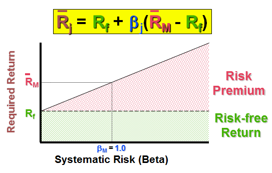
Obviously, with hindsight there was no need to calculate the required return for C plc as it has a beta of one and therefore the same level of risk as the market and will require the same level of return as the market, i.e. the RM of 11%. The systematic risk-return relationship is graphically demonstrated by the security market line. The CAPM contends that the systematic risk-return relationship is positive (the higher the risk the higher the return) and linear. Following diagrams shows the details;

It is understood that the risk-return relationship should be positive but it is hard to accept that in complex and dynamic world that the relationship will neatly conform to a linear pattern and there are doubts about the accuracy of the CAPM (Lynch, 2004).
Meaning of beta
The CAPM contends that shares co-move with the market. If the market moves by 1% and a share has a beta of two, then the return on the share would move by 2%. The beta indicates the sensitivity of the return on shares with the return on the market. Some companies' activities are more sensitive to changes in the market such as luxury car manufacturers have high betas, while those relating to goods and services likely to be in demand irrespective of the economic cycle such as food manufacturers have lower betas. The beta value of 1.0 is the benchmark against which all share betas are measured (Lynch, 2004).
If the Beta > 1 which is aggressive shares or Bull market which means that these shares tend to go up faster than the market in a rising (bull) market and fall more than the market in a declining (bear) market. If the Beta < 1 which is defensive shares or bear market these shares will generally experience smaller than average gains in a rising market and smaller than average falls in a declining market. If the Beta = 1 which is neutral shares or normal market these shares are expected to follow the market. Below diagrams show the characteristic lines and different Betas.


The beta value of a share is normally between 0 and 2.5. A risk-free investment (a treasury bill) has a β = 0 (no risk). The most risky shares like some of the more questionable penny share investments would have a beta value closer to 2.5. Hence, if the beta value is 11, it will be a mistake (Lynch, 2004).
3.5 Application of CAPM
1. Capital investment decisions
Calculation of cost of equity in the WACC calculation is used to enable an NPV calculation. A shareholder’s required return on a project will depend on the project’s perceived level of systematic risk. Different projects generally have different levels of systematic risk and therefore shareholders have a different required return for each project. A shareholder's required return is the minimum return the company must earn on the project in order to compensate the shareholder. It therefore becomes the company's cost of equity. Suppose ABC plc is evaluating a project which has a beta value of 1.5. The return on the FTSE All-Share Index is 15%. The return on treasury bills is 5%. Then the cost of equity will be = 5 + (15 - 5) 1.5 = 20% (Lynch, 2004).
2. Stock market investment decisions
The CAPM is one method that may be employed by analysts to help them reach their conclusions. An analyst would calculate the expected return and required return for each share. They then subtract the required return from the expected return for each share, i.e. they calculate the alpha value (or abnormal return) for each share. They would then construct an alpha table to present their findings. Suppose, when investing in ABC plc or XYZ plc the Beta value and expected return of ABC plc are 1.5 and 18% and Beta value and expected return of XYZ plc are 1.1 and 18% respectively. The market return is 15% and the risk-free return is 5%.
Required rate of return for ABC plc = 5 + 1.5(15 - 5) = 20% and Alpha value = 18-20= -2%
Required rate of return for XYZ plc = 5 + 1.1(15 - 5) = 16% and Alpha value = 18-16= 2%
It is advised to sell shares in ABC plc as the expected return does not compensate the investors for its perceived level of systematic risk, it has a negative alpha. Buy shares in XYZ plc as the expected return more than compensates the investors for its perceived level of systematic risk, i.e. it has a positive alpha (Lynch, 2004).
3. The preparation of an alpha table for a portfolio
The expected return of the portfolio is calculated as normal (a weighted average) and goes in the first column in the alpha table. Next is to calculate the required return of the portfolio. To do this it is required to calculate the portfolio beta, which is the weighted average of the individual betas. Then calculate the required return of the portfolio using the CAPM formula. Suppose the expected return of the portfolio A + B is 20%. The return on the market is 15% and the risk-free rate is 6%. 80% of your funds are invested in A plc and the balance is invested in B plc. The beta of A is 1.6 and the beta of B is 1.1 (Lynch, 2004).
Alpha value for the Portfolio (A + B) is shown below;
Bet value for (A + B) = (1.6 × .80) + (1.1 × .20) = 1.5
Required return for (A + B) = 6 + (15 - 6) 1.5 = 19.50%
Alpha value for Portfolio (A + B) = 20 - 19.50 = 0.50%
Alpha Value
If the CAPM is a realistic model and the stock market is efficient then the alpha values reflect a temporary abnormal return. In an efficient market, the expected and required returns are equal, i.e. a zero alpha. Investors are exactly compensated for the level of perceived systematic risk in an investment, i.e. shares are fairly priced. Arbitrage profit taking would ensure that any existing alpha values would be on a journey towards zero (Lynch, 2004).
The positive alpha of shares would encourage investors to buy shares. As a result the demand increases, the current share price would increase thus the expected return would fall. The expected return would keep falling and the level of the required return and the alpha will become zero. The negative alpha of shares would encourage investors to sell these shares. As a result the supply increases, the current share price would decrease thus the expected return would increase until it reaches the level of the required return and the alpha value becomes zero. The alpha values are dynamic as the share price. The alpha values may exist because CAPM does not perfectly capture the risk-return relationship due to the various problems with the model (Lynch, 2004).
3.6 Problems with CAPM
1. CAPM assumes that all the company's shareholders hold well-diversified portfolios and therefore need only consider systematic risk. However, a considerable number of private investors in the UK do not hold well-diversified portfolios (Lynch, 2004).
2. CAPM is a one period model, while most investment projects tend to be over a number of years (Lynch, 2004).
3. CAPM assumes the stock market is a perfect capital market. This is based on the following unrealistic assumptions. They are no individual dominates the market, all investors are rational and risk-averse, investors have perfect information, all investors can borrow or lend at the risk-free rate and no transaction costs (Lynch, 2004).
4. CAPM does not correctly express the risk-return relationship in some circumstances such as for small companies, high and low beta companies, low PE companies, and certain days of the week or months of the year (Lynch, 2004).
5. A scatter diagram is prepared of the share's historical risk premium plotted against the historical market risk premium usually over the last five years. The slope of the resulting line of best fit will be the β value. The difficulty of using historic data is that it assumes that historic relationships will continue into the future. This is questionable, as betas tend to be unstable over time (Lynch, 2004).
6. Richard Roll (1977) criticized CAPM as untestable, because the FTSE All-Share Index is a poor substitute for the true market, i.e. all the risky investments worldwide. How can the risk and return of the market be established as a whole? What is the appropriate risk-free rate? However, despite the problems with CAPM, it provides a simple and reasonably accurate way of expressing the risk-return relationship. CAPM is not perfect but it is the best model that we have at the moment. Moreover, some critics believe that the relationship between risk and return is more complex than the simple linear relationship defined by CAPM (Lynch, 2004).
3.7 APM formation
The arbitrage pricing model attempts to identify all of the macro-economic factors and then specifies how each factor would affect the return of a particular share. The APM is more sophisticated than CAPM in that it attempts to identify the specific macro-economic factors (inflation, industrial production, market risk premiums, interest rates, oil prices) that influence the return of a particular share (Lynch, 2004).
Each share will have a different set of factors and a different degree of sensitivity (beta) to each of the factors. To construct the APM for a share it requires the risk premiums and the betas for each of the relevant factors (Lynch, 2004).
Return on a share = RF + Risk premium F1.b +Risk premium F2.b2 + Risk premium F3.b3 + . . .
Such as Beta 1 = the effect of changes in interest rates on the returns from a share and Beta 2 = the effect of oil prices on the returns from a share (Lynch, 2004).

The pricing theory specifies asset (stock or portfolio) returns as a linear function of the aforementioned factors. APT gives the expected return on asset i as:
E(Ri) = Rf + b1*(E(R1) - Rf) + b2*(E(R2) - Rf) + b3*(E(R3) - Rf) + ... + bn*(E(Rn) - Rf)
Here:
Rf = Risk free interest rate (i.e. interest on Treasury Bonds)
bi = Sensitivity of the asset to factor i
E(Ri) - Rf) = Risk premium associated with factor i where i = 1, 2,...n
A share in a retail furniture company may have a high beta 1 and a low beta 2 whereas a share in a haulage company may have a low beta 1 and a high beta 2. Under the APM, these differences can be taken into account. However, despite its theoretical merits, APM scores poorly on practical application. The main problem is that it is extremely difficult to identify the relevant individual factors and the appropriate sensitivities of such factors for an individual share. This has meant that APM has not been widely adopted in the investment community as a practical decision-making tool despite its intuitive appeal (Iyer, n.d.).
3.8 Assumptions of APM
The arbitrage pricing theory is based on a number of assumptions. They are as follows:
1. The pricing theory assumes that asset/portfolio returns can be described by a multi-factor model and proceeds to derive the expected returns relation that follows from that assumption.
2. Since the intention is to maximize returns, the investor holds a number of securities so that unsystematic risk becomes negligible.
3. In time, arbitrageurs will exhaust all potential opportunities for riskless profits and the market will be in equilibrium (Iyer, n.d.).
3.9 Calculation of Portfolio Arbitrage
Let us assume that an investor has 2 portfolios A and B Where:
Expected return on portfolio A or E(RA) is 20%
βA or the systematic risk of portfolio A is 1.5
Expected return on portfolio B or E(RB) is 10%
βB or the systematic risk of portfolio B is 1
Consider portfolio C where E(RC) = 20% and βC = 1.2. Since portfolio C yields the same return as A but is less risky as evidenced by its systematic risk, an arbitrage profit should be possible. If we construct a portfolio D by allocating weights to Portfolio A and B in proportion of 40% and 60% then,
E(RD) = 0.4×E(RA) +0.6×E(RB) = 0.4×0.2 +0 .6×0.1 = 14%
βD = 0.4×βA + 0.6×βB = 0.4×1.5 +0.6× 1 = 1.2
Both portfolio C and D have the same level of risk but generate different returns. Thus, an arbitrageur can profit by shorting D and by using the proceeds of the short sale to buy portfolio C. Since the arbitrage pricing model gives the expected price of an asset, arbitrageurs use arbitrage pricing theory to identify and profit from mispriced securities (Iyer, n.d.).
4.0 Comparison of CAPM and APM
4.1 Similarities
Similar to the CAPM, the APT also assumes that there is a relationship between the risk and return of a portfolio (Rasiah et al., 2011).
CAPM and APT have several assumptions when using the formulae.
They both use a formula to measure returns in order to find which kinds of outcome need to be yielded in investing actions (Rasiah et al., 2011).
Both of them are methods of exploring the relationship between investment risk and potential returns on equity markets and they all use risk-free rate as a part of its formula (Rasiah et al., 2011).
The both models make definite assumptions that reach to same results. These assumptions are the capital market is perfect without any issue, investors have homogeny expectations: they claim they share the same understanding of risk and earning for an asset that is given to all investors and there is a linear relationship with the expected return and risk (Li & Zhang, 2012).
If there is a well-diversified portfolio, both model rule out the firm specific risk or unsystematic risk (Li & Zhang, 2012).
4.2 Differences
The major difference is CAPM uses only a single factor in determining the return of a portfolio, namely the beta of the portfolio. In other words, the non-diversifiable risk of the portfolio (in relation to the market risk) is the sole determinant of its return. No other factors will have any effect on the portfolio’s return. To address this criticism of the CAPM, the arbitrage pricing theory (APT) has been developed (Li & Zhang, 2012).
The potentially large number of factors means more betas to be calculated. There is also no guarantee that all the relevant factors have been identified. This added complexity is the reason arbitrage pricing theory is far less widely used than CAPM (Li & Zhang, 2012).
The APT is based on the concept of arbitrage (or law of one price), which states that any two identical investments cannot be sold at a different price. In other words, the theory states that market forces will adjust to eliminate any arbitrage opportunities, where a zero investment portfolio can be created to yield a risk-free profit. The key thing need to understand is that, unlike the CAPM, the APT does not assume that the market risk is the only factor that influences the return of a portfolio. The APT recognizes that several other factors (or risks) can influence the return of a portfolio (Li & Zhang, 2012).
The APT preserves the linear relationship between risk and return of the CAPM but abandons the single measure of risk by the beta of the portfolio. The APT model is a multiple factor model, which uses factors such as the inflation rate, the growth rate of the economy, the slope of the yield curve, etc. in addition to the beta of the portfolio in determining the return of the portfolio. Keep in mind that just as in the case with the CAPM, the APT can also be modified to determine the return of an individual investment (Li & Zhang, 2012).
In comparing to the CAPM, the APT has fewer assumptions. To building the APT requires only 3 assumptions, while the CAPM have more assumptions. The assumptions that are required for the CAPM but not for the APT are a single-period investment horizon, borrowing and lending at the risk-free rate and investors are mean-variance optimizer (Li & Zhang, 2012)
The systematic risk or market risk determines the expected rate of return in both model, however in the APT, there are non-diversifiable factors to affect the expected return on portfolio (Li & Zhang, 2012).
Even though both theories make the realistic assumptions of “investors would rather bigger property than less and avoid risk”, the quadratic utility assumption of the original CAPM is much more limiting compared to the APT (Li & Zhang, 2012)
In the APT, different than the CAPM, there is no need for the assumption of normal distribution of earnings with many variables. The APT does not make the probability distribution and does not assume that investors choose the portfolios according to expected earnings and variance or standard deviation (Li & Zhang, 2012)
The CAPM requires the market portfolio whilst the APT does not need it. Because of the difficulties that combine with market portfolio, the APT does not give credit to conditions as defining market portfolio or assignee. However; to have a applicable assignee for systematic risk factors, expected earning of a portfolio (a market index) is chosen (Dr. Boehme, n.d.).
The CAPM considers the conditional of risk free asset necessary with respect to the APM. The APT’s beta coefficient fairly allows some risk factor and the APT is more realistic when considering CAPM has only one beta coefficient (Dr. Boehme, n.d.).
The APT could be applied both single period and multi period while the CAPM is with one period (Dr. Boehme, n.d.).
The formula used for both models are very different. The formula used in CAPM is E(Ri) = Rf +Bi[Rm - Rf] whereas the formula used for the APT is E(RIBM) = Rf + BIBM,1[R1 - Rf] + BIBM,2[R2- Rf] + BIBM,3[R3 - Rf] …. (Dr. Boehme, n.d.).
5.0 Conclusion
Before making decision, suitable model selection depends on the sort of financial investments. However, it is significant to ask two fundamental questions for my personal decision about the model selection: How does an asset pricing model measure the risk of asset? How does an asset pricing model calculate the required return on assets?
Conceptually and theoretically, the APT can be taken in to consideration as an advanced version of the CAPM. However, the APT does not work as required in the practice, although it has more realistic assumptions and is more flexible(less restrictive) and strong. The APT does not mention how many risk factors or what type of factors we ought to use to measure risk in the model with regard to first question. In this case, causes to obstruct the model to compute efficiently the returns on asset because of the difficulty of determining the factors. The issues of factor can induce to higher prediction error and greater computation mistake. In addition, the APT is not easy to understand and apply from investment managers.
The CAPM is widely used and accepted as an asset pricing model by the financial management field. Even though It has more restrictive and limitations, it is easily applied by the financial investors and managers. The CAPM reflects the systematic risk much better and more substantial on the assets than the APT in terms of measuring risk. Furthermore, it generates a robust link between return and risk and so that this state is likely to provide lower estimation mistake. It is usually seen as a better model of calculating the required return on assets. Overall, the CAPM is simpler model and easier to understand and employ compared to the APT.
Therefore, the CAPM is more suitable on account of the model selection, since its responses to above-mentioned questions is more reasonable and understandable. In addition, another criteria to select the CAPM is that it is more useful the investment and financial management field. Nevertheless, the APT is new theory, because of this it is required to make more research and tests on the APT to prove itself.
In a nutshell, the CAPM and the APT let us to determine and measure the link between return and risk with the different and similar ways. Principally, even though both models are established as general equilibrium models of assets pricing, in the portfolio management they are widely used for the financial assets selection. The CAPM deduces that the only one element to determine the expected rate of return of assets lies on the relationship with each asset and their average market returns by using some assumptions and mean variance analysis. This relationship indicates the systematic risk and it measures with the beta coefficient in the model.
6.0 References
Dr. Boehme, R. (n.d.). CHAPTER 11: Arbitrage Pricing Theory (APT). Retrieved October 02, 2013 from
Hill, R. A. (2010). The Capital Asset Pricing Model. London, United Kingdom: Robert Alan Hill & Ventus Publishing ApS.
Iyer, A. (n.d.). Arbitrage Pricing Theory. Retrieved October 03, 2013, from http://www.buzzle.com/articles/arbitrage-pricing-theory.html
Li, Q. & Zhang, L. (2012). Comparing CAPM and APT in the Chinese Stock Market (Master thesis). Umeå University, Umeå, Sweden.
Lynch, P. (2004). The risk and return relationship part 2 – CAPM. Retrieved October 01, 2013, from http://www.accaglobal.com/en/student/acca-qual-student-journey/qual-resource/acca-qualification/p4/technical-articles/risk-return.html
Rasiah, D., et al. (2011). The effectiveness of arbitrage pricing model in modern financial theory. IJER, 2(3), 125-135.
Sufar, S. B., Ramlee, S., Ibrahim, I., Yusof, M. Z., & Yaacob, M. H. (2011). Investment analysis. Malaysia: Meteor Doc. Sdn. Bhd.
No comments:
Post a Comment
Note: Only a member of this blog may post a comment.